Frequently Asked Questions
A. General Overview
Q1: What is fracture imaging technology?
Fracture imaging technology is a suite of proprietary algorithms designed to detect and visualize fractures created during the stimulation of unconventional reservoirs. It uses microseismic events as high-frequency sources for reflection imaging. The technology provides high-resolution images of both newly created and pre-existing fractures and offers valuable insights into fracture growth. It can be applied to data recorded by both downhole sensors and Distributed Acoustic Sensing (DAS) arrays.
Q2: What type of imaging algorithm are you using?
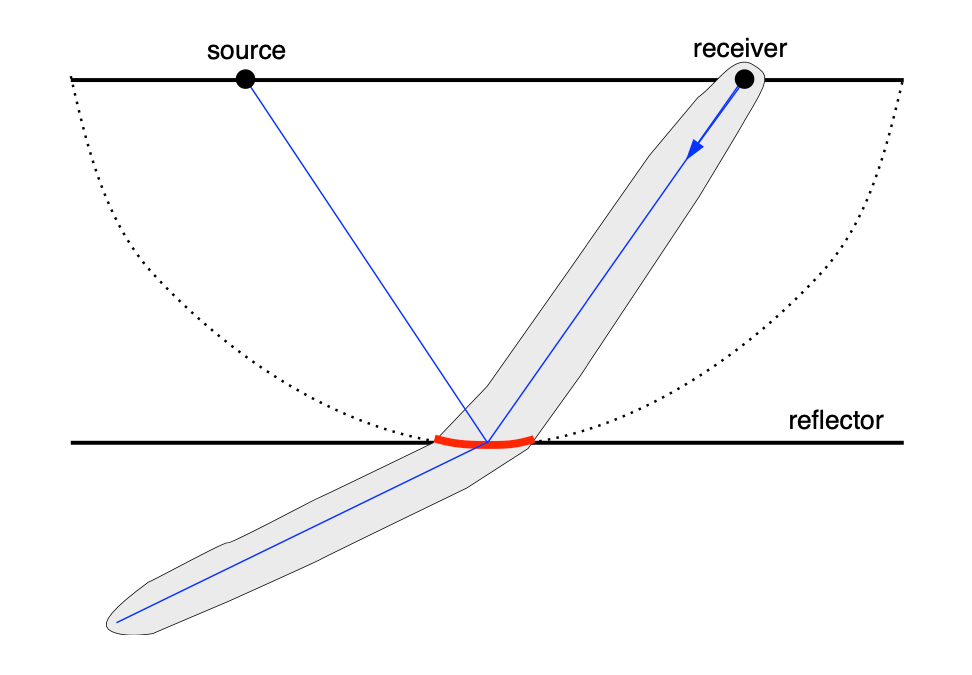
We use a modified version of the Fresnel-Volume Migration method originally presented in Luth et al. [2005]. This technique extends pre-stack Kirchhoff depth migration by incorporating wavefield polarization information to restrict the migration operator to the vicinity of the actual reflection point.
This approach helps resolve spatial ambiguities caused by limited aperture and low spatial coverage. For each seismic trace, we compute the direction of wave propagation, trace the ray back into the subsurface, and identify where it intersects the Kirchhoff summation surface at travel time t. We then calculate the Fresnel zone along the ray and determine the Fresnel radius at the reflection point, which defines the size of the reflector.
Fresnel-Volume Migration significantly reduces migration artifacts, particularly in low-aperture datasets. Because the imaging operator is frequency-dependent, it adapts naturally to a wide range of microseismic reflection data.
B. Signal Quality and Data Sufficiency
Q3: How can you justify that there is enough signal to pull from background noise and generate a reasonable image, particularly away from sensor array?
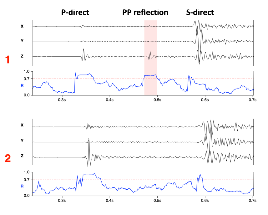
After signal processing and noise suppression, we perform hodogram analysis and compute linearity coefficients (R) for each sensor over time. These linearity values help identify portions of the microseismic waveform where the wave propagation direction can be reliably estimated and used for imaging.
By selecting only these high-quality signal segments, we significantly reduce background noise and minimize migration artifacts in the final image, even at distances away from the sensor array.
The Figure illustrates this procedure. A valid PP reflection is extracted from Seismogram 1, where the linearity values exceed the threshold (R = 0.7), indicated by the shaded red bars. This reflection data is then passed on for imaging. No reflection data is extracted from Seismogram 2.
Q4: What is relationship between signal to noise ratios of image and number of source events?
A higher number of source events improves image detail and reduces imaging artifacts through the constructive interference of reflections from different source-receiver pairs.
However, even a small number of high-quality events can produce an accurate image. Fewer sources result in a smaller illuminated area. From our experience, 30–50 high-quality events from a single stage are typically sufficient to generate a valid stage-level fracture image.
For typical geometries where the vertical array is positioned at the heel, we do not observe significant degradation in image quality between early and late stages. Early stages, while involving longer ray paths, are illuminated by a larger number of events. In contrast, late heel-ward stages have shorter ray paths but fewer contributing events. In such cases, the effects of energy loss along the wave path and the varying number of contributing source events tend to compensate for each other, maintaining consistent image quality across stages.
C. Reflection Data Processing
Q5: How do you separate the direct wavefield from the scattered wavefield used in the imaging?
We separate the direct wavefield by muting it based on arrival time picks or computed travel times. When time picks are available, we use them directly to mute the direct arrivals. For traces without time picks, we calculate synthetic travel times using the velocity model and apply muting based on these computed arrival times. This process effectively isolates the scattered wavefield, which is then used for imaging.
Q6: How do you account for the effects of varying source mechanisms and radiation patterns in microseismic data?
When moment tensor inversion (MTI) solutions are not available, we use a stacking approach based on the absolute amplitudes of the reflection data. This method allows us to apply imaging even when the radiation patterns of the microseismic events are unknown. The input to the imaging procedure includes the source-receiver pair location and the recorded waveform. For each trace, we normalize its amplitude to the maximum energy within that trace. This prevents stronger events from dominating the final image and obscuring contributions from smaller events.
While this normalization reduces the resolution of the final image, it increases its stability—especially in the presence of uncertainties in event location or source mechanism.
When MTI solutions are available, we can perform true amplitude imaging. This involves compensating for the radiation pattern of each microseismic source before applying the imaging operator. Proper radiation pattern compensation allows us to compute reflection coefficients for fractures, which can in turn help to differentiate between fluid-filled and proppant-filled fractures based on their reflective behavior.
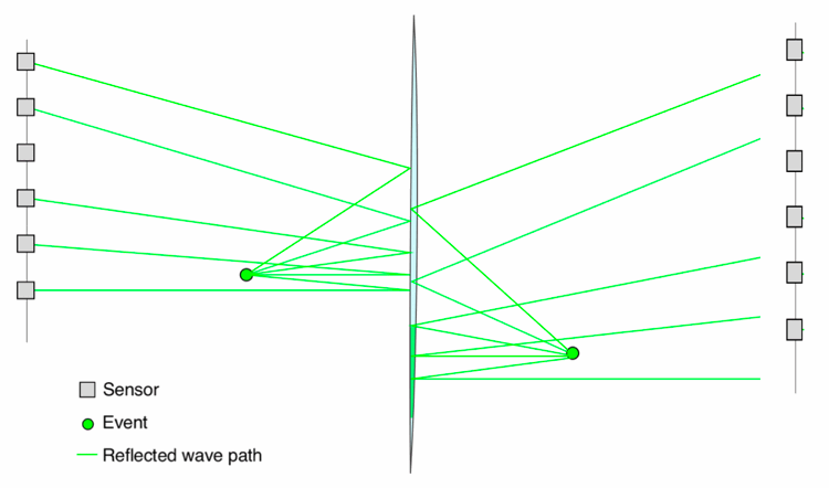
Q7: How do you deal with imaging reflectors using sources from both sides of a reflector?
For absolute amplitude processing, we normalize each trace to account for amplitude decay between the receiver and the reflection point. Each contributing source-receiver pair in each sensor array is processed individually, and their results are then merged. This merging process helps to optimize the imaged fracture's position and geometry by using data from both sides of the reflector.
For true-amplitude processing, we compute the reflection coefficient for each source-receiver pair. Each pair contributes a reflection coefficient value projected into the Fresnel Zone of the reflector. This process is performed for both sensor arrays, providing a rich and spatially varying measure of reflection coefficients across the imaged fracture.
This capability to compute localized reflection coefficients serves as the input data for distinguishing between different fracture fill types—specifically, helping to separate fluid-filled from proppant-filled regions of the fracture.
D. Imaging Accuracy and Artifacts
Q8: How does the uncertainty in the location of the microseismic events effect the image?
We can consider 3 different scenarios:
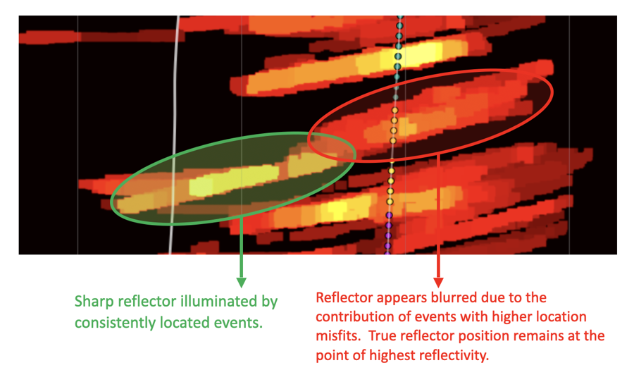
1. Reflector is well illuminated by a large number of events. Event population includes high and low confidence events.
Reflector is well illuminated by a large number of events, including both high- and low-confidence locations. In this case, the true position of the reflector is confirmed by the stacking of reflection data from accurately located events. Events with poorer location accuracy contribute a small amount of blur around the true reflector position but do not affect the overall accuracy of the reflector geometry.
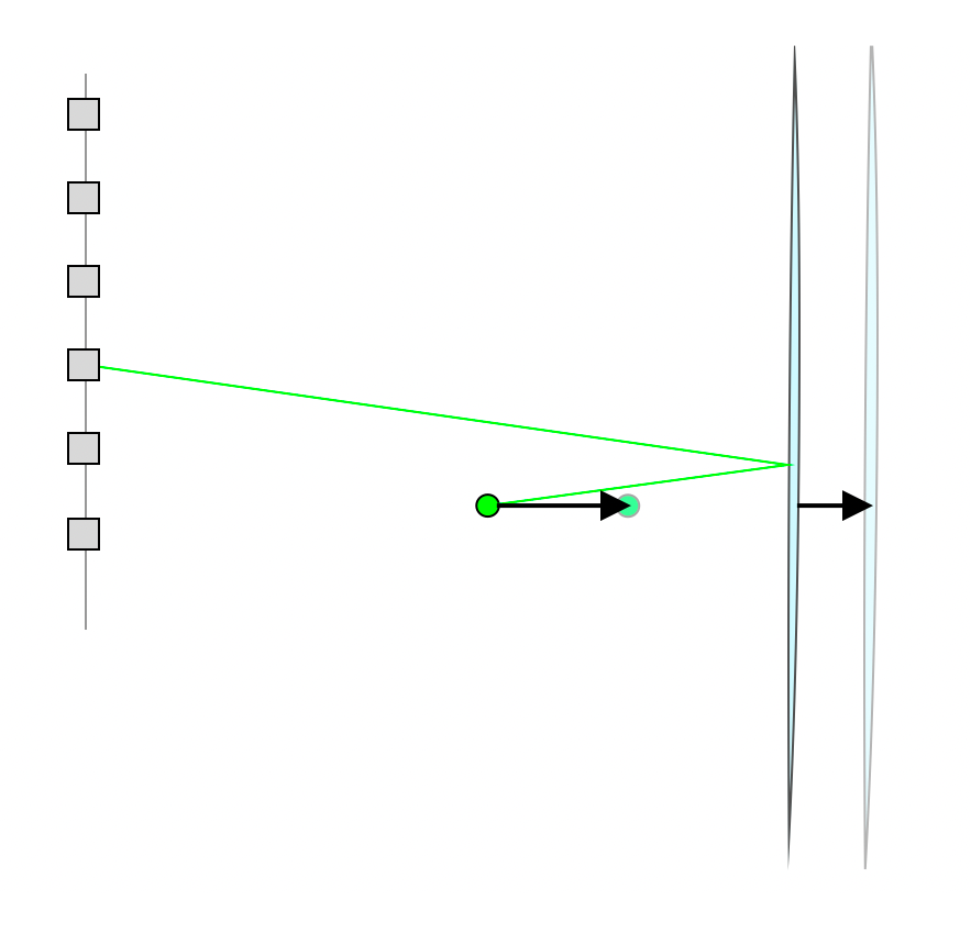
2. Event locations are consistently shifted due to an error in velocity model.
In this situation, the reflector will appear displaced, but the overall geometry of the reflector remains correct.
Typically, both the events and the reflectors are shifted either toward or away from the receiver array. Importantly, the displacement of the reflector is approximately half of the shift experienced by the event locations.
Even with this shift, we can still sharpen the final image by constraining the source-receiver pairs to illuminate the existing reflector structure, although this approach will not add finer details to the image.
A critical point is that if the velocity model error exceeds half of the dominant period of the microseismic data, it can cause destructive interference during stacking, as reflections with opposite polarities are back-projected into the subsurface.
For example, for a dominant P-wave frequency of 300 Hz, the acceptable time pick misfit must be no greater than 1.7 milliseconds to avoid polarity reversal. This level of accuracy is routinely achievable using a full VTI (Vertical Transversely Isotropic) velocity model that has been calibrated with known perforation shots.
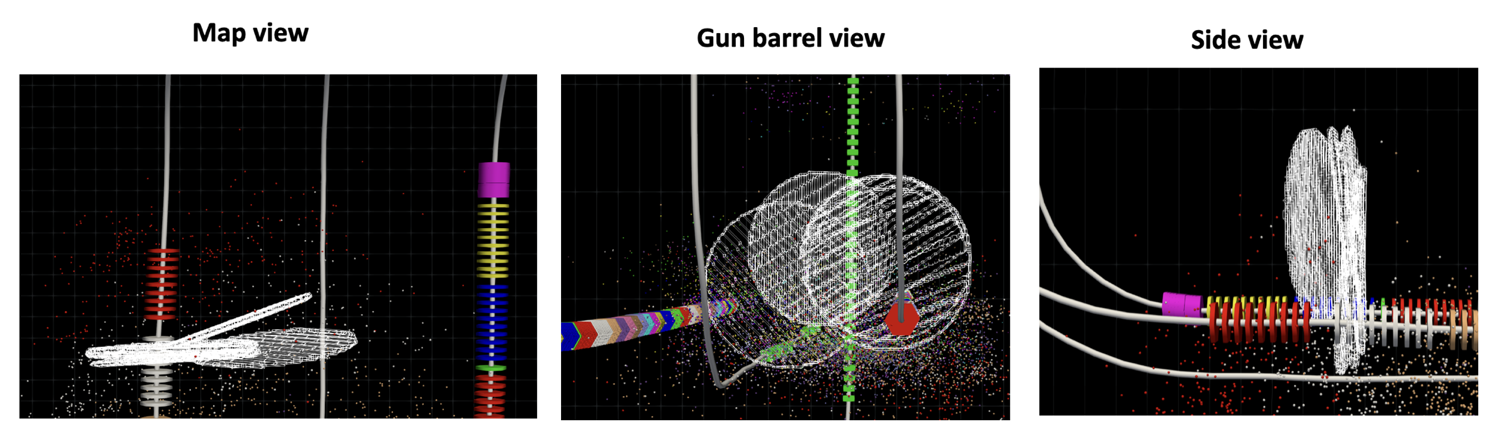
3. Reflector is illuminated by a small number of events.
This situation typically occurs at greater distances or offsets from the sensor array, where only a limited number of events can effectively illuminate the target stages.
In this case, the reflector may appear as a single 3D disk or a series of thin, parallel disks in the image. While the overall geometry of the reflector is still preserved, the accuracy of its position becomes less reliable, and the illuminated area may be restricted. Based on our experience, approximately 30–50 high-quality events are required to sufficiently stabilize the position and orientation of a reflector to achieve a reliable and interpretable image.
Q9: How do you deal with the artifacts in the image caused by the non-uniform source distribution?
We address this issue by analyzing the number of microseismic sources contributing to each part of the image. This enables us to compute a compensation factor that reduces artifacts arising from uneven source coverage.
Additionally, we correct for energy loss along the wave path—both from the source to the reflector and from the reflector to the receiver. These adjustments help ensure that variations in image brightness are due to actual reflectivity rather than geometric or propagation effects.
In the plot, one can see a horizontal section of the image computed using a single vertical sensor array, located at the top of the plot (marked by a green circle). The maximum distance between the sensor array and the imaged reflector is approximately 5,500 ft. Notably, even though the early toe-ward stages (in the lower part of the plot) have significantly fewer contributing events, there is no systematic degradation in reflectivity. This illustrates the effectiveness of our artifact mitigation approach.
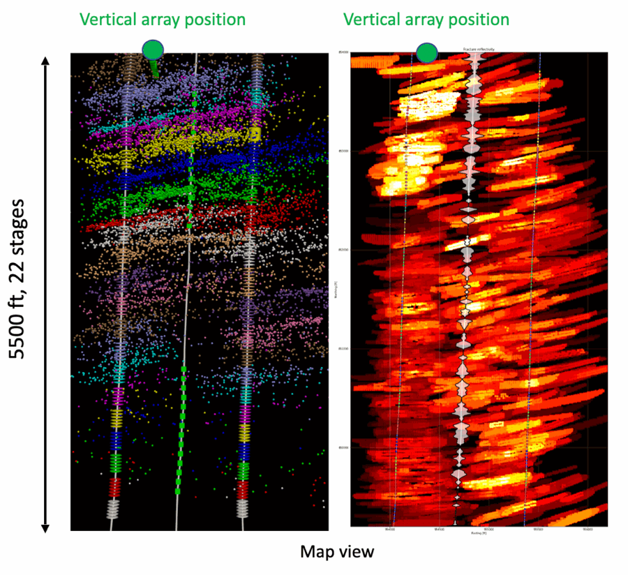
In this example, we also have access to permanent fiber data, which allows us to calibrate the reflectivity threshold to achieve the best agreement between observed and imaged fracture features, while minimizing migration artifacts.
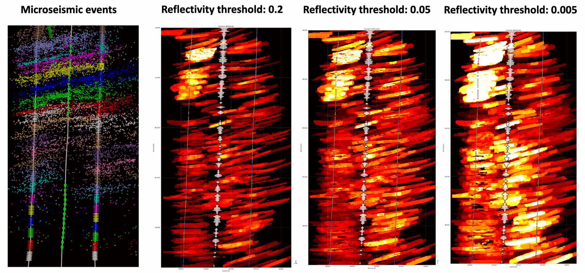
In the plot below, we show how reflectivity thresholds can be tuned using external diagnostics. For instance, frac hits observed on other tools—such as pressure communication or cross-well strain measurements—can be used to validate and fine-tune imaging parameters. This cross-verification significantly improves the reliability of the final fracture image, especially in areas with limited source coverage or weak reflectivity.
E. Reflector and Fracture Characterization
Q10: How do you separate the bedding plane reflections from the events reflecting off the fractures?
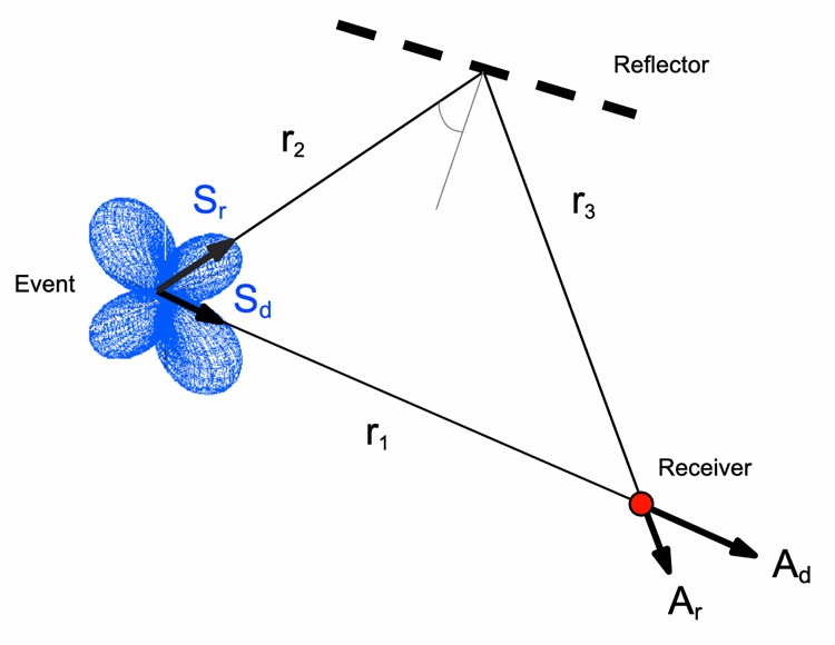
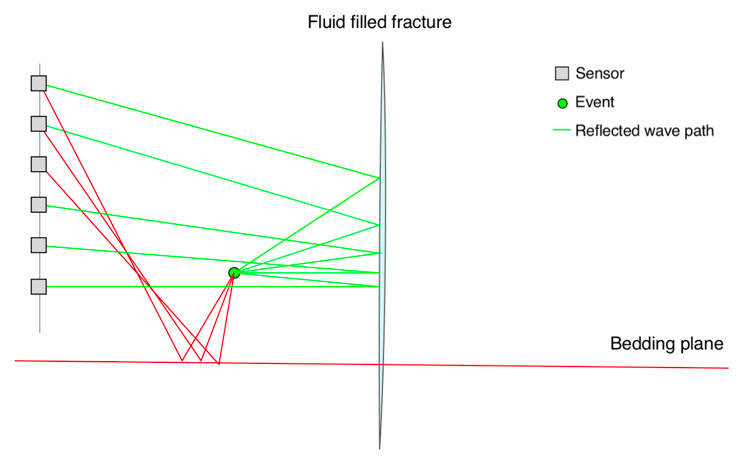
Our imaging algorithm leverages polarization information to distinguish between reflections from different geological features (see Q2 for more details).
Specifically, reflections from sub-horizontal bedding planes and sub-vertical, fluid-filled fractures exhibit distinctly different polarization characteristics. These differences are used to separate the two types of reflections during the imaging process. As illustrated in the figure, the polarization vectors for bedding plane reflections are generally horizontal, while those from vertical fractures are more vertically polarized or exhibit a different angular distribution, depending on the geometry and wave mode.
This polarization-based separation significantly reduces ambiguity between structural and fracture-related features.
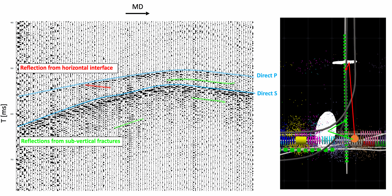
Bedding plane reflections typically exhibit flat or gently curving move-out patterns and sub-vertical P-wave polarizations, while reflections from sub-vertical fractures show steeper move-out curves and distinct, often sub-horizontal or oblique P-wave polarizations.
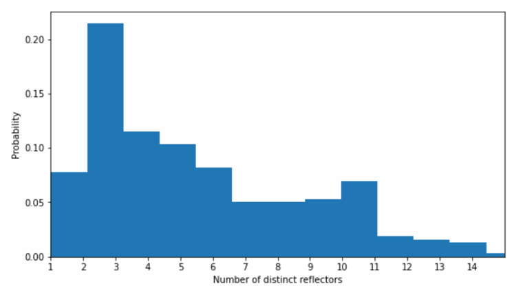
Q11: How many distinct fractures can you detect using a single microseismic source?
We evaluated the number of reflections from distinct fractures for multiple microseismic sources under optimal conditions, using a high-aperture vertical array positioned at the target depth and located near the heel, within the stimulated volume.
For the HFTS2 dataset, we analyzed only those events that contributed to the final image. A histogram showing the number of distinct fractures detected by individual microseismic events is shown in the figure. This analysis demonstrates that a single well-positioned microseismic event can illuminate 2-6 distinct fracture surfaces.